Chi-Square Test
The chi-square test (KHGR2) is the most commonly used method for comparing frequencies or proportions. It is a statistical test used to determine if observed data deviate from those expected under a particular hypothesis. The chi-square test is also referred to as a test of a measure of fit or "goodness of fit" between data. Typically, the hypothesis tested is whether or not two samples are different enough in a particular characteristic to be considered members of different populations. Chi-square analysis belongs to the family of univariate analysis, i.e., those tests that evaluate the possible effect of one variable (often called the independent variable) upon an outcome (often called the dependent variable).
The chi-square analysis is used to test the null hypothesis (H0), which is the hypothesis that states there is no significant difference between expected and observed data. Investigators either accept or reject H0, after comparing the value of chi-square to a probability distribution. Chi-square values with low probability lead to the rejection of H0 and it is assumed that a factor other than chance creates a large deviation between expected and observed results. As with all non-parametric tests (that do not require normal distribution curves), chi-square tests only evaluate a single variable, thus they do not take into account the interaction among more than one variable upon the outcome.
A chi-square analysis is best illustrated using an example in which data from a population is categorized with respect to two qualitative variables. Table 1 shows a sample of patients categorized with respect to two qualitative variables, namely, congenital heart defect (CHD; present or absent) and karyotype (trisomy 21, also called Down syndrome, or trisomy 13, also called Patau syndrome). The classification table used in a chi-square analysis is called a contingency table and this is its simplest form (2 x 2). The data in a contingency table are often defined as row (r) and column (c) variables.
In general, a chi-square analysis evaluates whether or not variables within a contingency table are independent, or that there is no association between them. In this example, independence would mean that the proportion of individuals affected by CHD is not dependent on karyotype; thus, the proportion of patients with CHD would be similar for both Down and Patau syndrome patients. Dependence, or association, would mean that the proportion of individuals affected by CHD is dependent on kayotype, so that CHD would be more commonly found in patients with one of the two karyotypes examined.
Table 1 shows a 2 x 2 contingency table for a chi-square test—CHD (congenital heart defects) found in patients with Down and Patau syndromes
Figure 1. Chi-square distributions for 1, 3, and 5 degrees of freedom. The shaded region in each of the distributions indicates the upper 5% of the distribution.
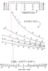
Chi-square is the sum of the squared difference between observed and expected data, divided by the expected data in all possible categories:
Χ2 = (O11 - E11)2 / E11 + (O12 - E12)2 / E 12 + (O21 - E21)2/ E21 + (O22–E22)2 / E22, where O11 represents the observed number of subjects in column 1, row 1, and so on. A summary is shown in Table 2.
The observed frequency is simply the actual number of observations in a cell. In other words, O11 for CHD in the Down-syndrome-affected individuals is 24. Likewise, the observed frequency of CHD in the Patau-syndrome-affected patients is 20 (O12). Because the null hypothesis assumes that the two variables are independent
| Karyotype | ||||
| Down syndrome | Patau syndrome | Total | ||
| Congenital Heart Defects | CHD present | 24 | 20 | 44 |
| CHD absent | 36 | 5 | 41 | |
| Total | 60 | 25 | 85 | |
| Karyotype | ||||
| Down syndrome | Patau syndrome | Total | ||
| Congenital Heart Defects | CHD present | O11 | O12 | r1 |
| CHD absent | O21 | O22 | r2 | |
| Total | c1 | c2 | N | |
| Observed (o) | Expected (e) | o-e | (o-e)2 | (o-e)2/e |
| 24 | 31.1 | -7.1 | 50.41 | 1.62 |
| 20 | 12.9 | 7.1 | 50.41 | 3.91 |
| 36 | 28.9 | 7.1 | 50.41 | 1.74 |
| 5 | 12.1 | -7.1 | 50.41 | 4.17 |
| 85 | 85.0 | Χ2=11.44 |
of each other, expected frequencies are calculated using the multiplication rule of probability. The multiplication rule says that the probability of the occurrence of two independent events X and Y is the product of the individual probabilities of X and Y. In this case, the expected probability that a patient has both Down syndrome and CHD is the product of the probability that a patient has Down syndrome (60/85 = 0.706) and the probability that a patient has CHD (44/85 = 0.518), or 0.706 x 0.518 = 0.366. The expected frequency of patients with both Down syndrome and CHD is the product of the expected probability and the total population studied, or 0.366 x 85 = 31.1.
Table 3 presents observed and expected frequencies and Χ2 for data in Table 1.
Before the chi-square value can be evaluated, the degrees of freedom for the data set must be determined. Degrees of freedom are the number of independent variables in the data set. In a contingency table, the degrees of freedom are calculated as the product of the number of rows minus 1 and the number of columns minus 1, or (r-1)(c-1). In this example, (2-1)(2-1) = 1; thus, there is just one degree of freedom.
Once the degrees of freedom are determined, the value of Χ2 is compared with the appropriate chi-square distribution, which can be found in tables in most statistical analyses texts. A relative standard serves as the basis for accepting or rejecting the hypothesis. In biological research, the relative standard is usually p = 0.05, where p is the probability that the deviation of the observed frequencies from the expected frequencies is due to chance alone. If p is less than or equal to 0.05, then the null hypothesis is rejected and the data are not independent of each other. For one degree of freedom, the critical value associated with p = 0.05 for Χ2 is 3.84. Chi-square values higher than this critical value are associated with a statistically low probability that H0 is true. Because the chi-square value is 11.44, much greater than 3.84, the hypothesis that the proportion of trisomy-13-affected patients with CHD does not differ significantly from the corresponding proportion for trisomy-21-affected patients is rejected. Instead, it is very likely that there is a dependence of CHD on karyotype.
Figure 1 shows chi-square distributions for 1, 3, and 5 degrees of freedom. The shaded region in each of the distributions indicates the upper 5% of the distribution. The critical value associated with p = 0.05 is indicated. Notice that as the degrees of freedom increases, the chi-square value required to reject the null hypothesis increases.
Because a chi-square test is a univariate test; it does not consider relationships among multiple variables at the same time. Therefore, dependencies detected by chi-square analyses may be unrealistic or non-causal. There may be other unseen factors that make the variables appear to be associated. However, if properly used, the test is a very useful tool for the evaluation of associations and can be used as a preliminary analysis of more complex statistical evaluations.
Resources
Books
Grant, Gregory R., and Warren J. Ewens. Statistical Methods in Bioinformatics. New York: Springer Verlag, 2001.
Nikulin, Mikhail S., and Priscilla E. Greenwood. A Guide to Chi-Square Testing. New York: Wiley-Interscience, 1996.
Other
Rice University. Rice Virtual Lab in Statistics. "Chi Square Test of Deviations." (cited November 20, 2002). <http;://www. ruf.rice.edu/~lane/stat_sim/chisq_theor/>.
Antonio Farina
Additional topics
Science EncyclopediaScience & Philosophy: Categorical judgement to Chimaera